Showing posts with label box and whisker plots. Show all posts

Friday, June 26, 2009

Five number summary and box and whiskers plot

The five number summary does not list all the information, but instead lists the low value, Q1, Q2, Q3 and the high value. The Q's stand for quartile, which means Q1 is the split for the low 25% of the data, Q2 is the median and Q3 is the split for the high half of the data. You can think of Q1 and Q2 as the medians of the low half and the high half, respectively. The interquartile range or IQR is the distance from the third quartile to the first, which is Q3 - Q1.

Let's look at the list.

7 | 678
7 | 00111224
6 | 556666666688999
6 | 000122334

With 35 entries, the middle entry is the 18th, either counting from top to bottom or bottom to top. That is the 6 marked in red and bold, so Q2 = 66.

There are 17 entries in the top half and 17 in the low half, so the position of the high and low quartiles is 9 away from the top and 9 away from the bottom, respectively. These are marked in bold and blue, with Q1 = 64 and Q3 = 71.

The five number summary is as follows

High = 78
Q3 = 71
Q2 = 66
Q1 = 64
Low = 60

Now we draw the box and whiskers in three steps, shown in the picture.


The first step is to draw the box between the values for the first and third quartiles, with a dotted line at the second quartile. We also can put dots to mark the high and low values.

The next step is computing the Interquartile Range, IQR = Q3 - Q1, which in this case is 71-64 = 7. We mark boundaries called the threshold which will be 1.5 times IQR above the third quartile and 1.5 time IQR below the first quartile. In our case, this would be at 71+ 1.5*7 = 81.5 and 64 - 1.5*7 = 63.5.

The third step is checking for outliers, If the high and low values are within these thresholds, the whiskers extend to the high value to the right and the low value to the left. (Box and whiskers can also be drawn vertically, so change the directions to high an dlow in that case.) If all the data is inside, the whiskers extend all the way to high and low. If there is data outside, those count as outliers and the whiskers are drawn to the highest data inside the high threshold and the lowest data inside the low threshold. One this has been done, we erase the thresholds.

Wednesday, February 4, 2009

Class notes for 2/4

More on the five number summary and outlying data. Consider the number of wins for each team in the NFC at the end of the 2008 season. In order, the list looks like this.

12, 12, 11, 10, 9, 9, 9, 9, 9, 8, 8, 7, 6, 4, 2, 0

The five number summary is as follows.

High: 12
Q3 : 9.5
Q2 : 9
Q1 : 6.5
Low: 0

Now we check to see if any of the numbers are outliers.

IQR = 9.5 - 6.5 = 3
Q3 + 1.5*IQR = 9.5 + 4.5 = 14 (no data higher than this, so no high outliers)
Q1 - 1.5*IQR = 6.5 - 4.5 = 2 (the value 0 is a low outlier, the value 2 is just inside the threshold)

The Detroit Lions' total of no wins in 16 games was the low outlier in the NFC.

Here is the data for the AFC.

13, 12, 12, 11, 11, 11, 9, 8, 8, 8, 7, 5, 5, 4, 4, 2

The five number summary is as follows.

High: 13
Q3 : 11
Q2 : 8
Q1 : 5
Low: 2

Now we check to see if any of the numbers are outliers.

IQR = 11 - 5 = 6
Q3 + 1.5*IQR = 11 + 6 = 17 (no data higher than this, so no high outliers)
Q1 - 1.5*IQR = 5 - 6 = -1 (no data lower than this, so no low outliers)

Here are the two conferences' box and whisker plots shown above and below a scale that goes from 0 to 13.


Parameters and statistics for categorical data. We have already defined some numbers that are associated with data sets, which we call parameters if the data set is a population and statistics if the data set is a sample. Statistics has the idea of reserved symbols, like N and n for size of the data set, population and sample respectively, and mux and x-bar for the mean. With categorical data, the number of units that share a value for a given categorical variable is called the frequency of the value, denoted by F(value) in a population of f(value) in a sample. Two data sets with the same variable can be compared, but if the size of the sets is significantly different, it is fairer to compare the relative frequency, which if the frequency divided by the size of the data set, denoted by p in a population and p-hat in a sample.

For example, let's look at Data Set #2 and the variable of Major. Here are the frequencies of each value that has at least one subject.

f(AH) = 6
f(BF) = 13
f(CESM) = 2
f(HE) = 4
f(SS) = 4
f(Other) = 11
f(Und) = 2

To get the relative frequencies, we divide the frequencies by n, which in this case is 42. This gives us the p-hat values, which we will usually express as a percent. In the following equations, the symbol ~= means "approximately equal to".

p-hat(AH) = 6/42 ~= 14%
p-hat(BF) = 13/42 ~= 31%
p-hat(CESM) = 2/42 ~= 5%
p-hat(HE) = 4/42 ~= 10%
p-hat(SS) = 4/42 ~= 10%
p-hat(Other) = 11/42 ~= 26%
p-hat(Und) = 2/42 ~= 5%

The sum of all of relative frequency should give us 100%, but sometimes we get rounding error. In this case, the sum is 101%. When this happens, we round to the nearest tenth of a percent, hoping that the total will be either 99.9%, 100% or 100.1%. This is called the +/- .1% rule for rounding relative frequency.

p-hat(AH) = 6/42 ~= 14.3%
p-hat(BF) = 13/42 ~= 31.0%
p-hat(CESM) = 2/42 ~= 4.8%
p-hat(HE) = 4/42 ~= 9.5%
p-hat(SS) = 4/42 ~= 9.5%
p-hat(Other) = 11/42 ~= 26.2%
p-hat(Und) = 2/42 ~= 4.8%

The sum of the more closely rounded numbers is now 100.1%, which is close enough. With some sets of fractions that add up to 1, which in general are called probability distributions, it doesn't matter how far you go when rounding, you will never get exactly 100%, which is why we decide on this "close enough" method. For instance 1/3 + 1/3 + 1/3 = 1, but if we round 1/3 and then add them up, we get 99% or 99.9% or 99.99%, etc. depending on how far we round the numbers. Because these kinds of cases can show up, we decide on a fixed number we consider close enough, known in math as an epsilon value, and round all the numbers to the same number of digits after the decimal until the total is close enough.

Example of a worst case scenario: If we have 16 values for a variable and all the values show up once, every number in our probability distribution is 1/16 = .0625 = 6.25%

Rounded to nearest percent: 1/16 ~= 6%. 16*6% = 96%, way too low
Rounded to nearest tenth of a percent: 1/16 ~= 6.3%. 16*6.3% = 100.8%, too high
Rounded to nearest hundredth of a percent: 1/16 = 6.25%. Now the total is exactly 100%, since there is no rounding at all.

Monday, February 2, 2009

Class notes for 2/2

Graphical representation of data

Frequency tables and dotplots: A frequency table is a list of values, which we will call x, followed by the number of times each value shows up on the list, which is called the frequency, denoted by f or f(x). A dotplot is a graph that represents a frequency table. For example, let's take the frequency table from the last class notes and turn it into a dotplot with a vertical scale.

x || f(x)

20 || 2
19 || 1
18 || 2
17 || 5
16 || 7
15 || 2
14 || 5
13 || 5
12 || 3
11 || 5
_9 || 2
_8 || 1
_7 || 2
_4 || 3


For the dot plot version, I type in the information in the Courier font, which is mono-spaced. This was the same number of characters on a line will take up the same width

20| **
19| *
18| **
17| *****
16| *******
15| **
14| *****
13| *****
12| ***
11| *****
10|
9 | **
8 | *
7 | **
6 |
5 |
4 | ***
3 |
2 |
1 |

Notice that every value from 1 to 20 is included in the scale, even the ones that did not appear on the list. This is so the dotplot will be correctly spaced.

The five number summary, box and whiskers, IQR and outlying data. Examples of five number summaries and box and whisker plots can be seen in the previous class notes, but John Tukey added one more idea to the box and whisker definition, which would take into account the idea of outlying data, values that are far larger or far smaller than most of the other data. The question is how to define "far larger" and "far smaller", and we will see that in all the different systems we use, the cut-off point for these decisions is arbitrary. Tukey's arbitrary decision involves a number called the Inter-quartile Range or IQR for short. The formula is as follows:

IQR = Q3 - Q1

This is the distance between the values that define the cut-off points for the 75th percentile and the 25th percentile, so the middle half of the data lies inside that range. That is represented by the box, and Tukey decided that the neither the left or right whisker should ever be more than one and a half times as long as the width of the box. If there is any data that is higher that Q3 + 1.5*IQR, it is represented by a dot. Likewise, any data that is lower than Q1 - 1.5*IQR is represented by a dot. The whiskers only extend to the highest data less than the high outlier threshold or the lowest data more than the low outlier threshold.

Example: Here are the number of times the most popular twelve stories on the Huffington Post website were read today, where the scale is in thousands or readers.

759 165 162 152 132 129 128 118 113 65 55 44 35

Obviously, the most popular story* is being read by more people than the next five stories combined, so we would expect it to be outlying data. Let's create the five number summary, the IQR and find the outlier thresholds.

High: 759
Q3: 157 (The average of 162 and 152)
Q2: 128.5 (The average of 129 and 128)
Q1: 60 (The average of 65 and 55)
Low: 35

IQR = 157 - 60 = 97

High outlier threshold = Q3 + 1.5*IQR = 157 + 1.5*97 = 157 + 145.5 = 302.5
Low outlier threshold = Q1 - 1.5*IQR = 60 - 1.5*97 = 60 - 145.5 = -85.5

As we might expect, there is no low outlying data, but the highest value of 759 is much higher than any of the rest of the data. The way this will be presented is by the upper whisker only extending to the value of 165, which is the highest non-outlying value, while the outlier will be represented by a dot. Here is a horizontal box and whisker plot of this data. You can click on this picture to get a larger version.


(* The most popular story the day this data was taken were pictures of Olympic champion Michael Phelps smoking a bong in the dorm room of a friend.)

Rounding: There are several different rules for rounding values, depending on what the data looks like. In general, when taking data from a list and finding the average, we round to one decimal place more than the data is represented. If numbers are given as whole numbers, we round to the nearest tenth. If numbers are given to the nearest penny, we round the average to the nearest tenth of a penny.

The numbers I gathered from the website I decided to round to the nearest thousand then write the numbers in thousands. For this decision, I used the significant digit method. If you put too many places of numbers, people can get caught up in the precision of the number instead of the general size of the number. For big numbers reported in newspapers and magazines, most writers use either one or two or three significant digits, which is to say how many digits are reported before you round the rest of the number to zeroes.

Here are some examples. Let's say that the bailout of the banks cost $763,922,575,873.22. That's too much information, and who knows if being precise makes any sense, since the final numbers might change.

One significant digit: The bank bailout costs $800 billion.
Two significant digits: The bank bailout costs $760 billion.
Three significant digits: The bank bailout costs $764 billion.

All of these answers are correct, depending on how many significant digits we decide to use. The more significant digits, the more precise the answer is, but using more than three or so significant digits for data presented to the public is probably too much information. If we are using numbers in calculations, we usually want to be as precise as possible, and only do the rounding at the end, when the number is presented as the answer.

Order of operations: You may have learned the order of operations by remembering the word PEMDAS or the mnemonic device

Please (parentheses)
Excuse (exponents)
My Dear (multiplication and division)
Aunt Sally (addition and subtraction)

With calculators like the TI-30X II s or the TI-83 or TI-84, the display screen has a line which shows you the equation as you press the keys, so you can enter an entire equation just once and then press the [ENTER] key. The calculator understands the order of operations rules, but sometimes you still have to be careful how you type your formulas in.

A fraction is really two sets of parentheses. You might remember the formula for the slope of a line in algebra class as being the difference of the y values divided by the difference of the x values. Let's say the two points were (8, 7) and (4, 2). Because of the fraction sign we want to do 7-2 = 5 and 8-4 = 4 BEFORE we do the division, so to make that clear to the calculator, we have to put parentheses around the numerator equation, press the division key, then parentheses around the denominator equations, then press [ENTER].

On your calculator, the square root is followed by an open parentheses. In some texts, a formula that includes a square root might show two number being multiplied together by putting the numbers in parentheses and next to each other instead of using the multiplication sign. That can be a problem on the calculator, because the square root starts it own set of parentheses. Instead of typing (.3)(.7), on the calculator you should type .3*.7. The instructions for different equations are shown below.

On most calculators, you don't have to close every set of parentheses. The only calculator I know that is a stickler for parentheses agreeing with one another left and right is the TI-89. On the other hand, if you use a spreadsheet program, it will always complain if your left and right parentheses don't agree.


Thursday, January 29, 2009

Class notes for 1/28

More on frequency tables: When we have a lot of duplicate values in a data set, a frequency table lets us write that data more compactly, by listing each value x, followed by the positive number of times it shows up, f(x). Let's look at the data list from the 1/26 notes, which were the scores in one of the two classes this semester on the first quiz.

x || f(x)

20 || 2
19 || 1
18 || 2
17 || 5
16 || 7
15 || 2
14 || 5
13 || 5
12 || 3
11 || 5
_9 || 2
_8 || 1
_7 || 2
_4 || 3


We already discussed how to find the mode and median, but what about the mean? We need to find n, and we need to find the sum of all the x values. To get those numbers, n = sum(f(x)) and sum(x) = sum(x*f(x)). Here is the list again with another column of numbers added, the value multiplied by its frequency.

x || f(x) || x*f(x)

20 || 2 || 40
19 || 1 || 19
18 || 2 || 36
17 || 5 || 85
16 || 7 ||112
15 || 2 || 30
14 || 5 || 70
13 || 5 || 65
12 || 3 || 36
11 || 5 || 55
_9 || 2 || 18
_8 || 1 || _8
_7 || 2 || 14
_4 || 3 || 12

The sum of the second column is 45, the sum of the third column is 600, so x-bar=600/45=13.333..., or rounded to the nearest tenth, 13.3.
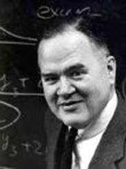

The ideas of John Tukey. John Tukey was a statistician and computer scientist who did a lot of his best work back in the 1960s. Many of his ideas in statistics are about easier and shorter ways to present data sets. We will study three of them, the stem and leaf plot, the five number summary and its graphical representation, the box and whiskers plot.

Stem and leaf plots. If we don't have a lot of duplication, a frequency table is not going to make presenting data any shorter. What Tukey did was split numbers into two parts, the stem and the leaf. The standard way to do this is to make the last digit the leaf and the rest of the number the stem. For example, the number 87 would have stem = 8 and leaf = 7. Tukey's idea was to put the stem numbers at the left and list the leaves from low to high, using a mono-spaced font, which back in the day of typewriters was the only choice available for someone typing. (Courier is a mono-spaced font. The letter i is the same width as the letter w or any other symbol. Most fonts used today aren't mono-spaced anymore, but in this situation, we want to use Courier.)

Here is a list of numbers. It is the number of wins by teams in the American League at the end of the 2008 regular season.

97, 95, 89, 86, 68, 89, 88, 81, 75, 74, 100, 79, 75, 61

The highest number is 100, so we make the stem 10 and the leaf 0. All the numbers on the list are put in stem and leaf form, where the stem is underlined and followed by a |, then the leaves are listed from low to high from left to right.

____
10 | 0
_9 | 57
_8 | 16899
_7 | 4559
_6 | 18


Sometimes data is too spread out to use the last digit as the leaf, and instead the last two digits are the leaf, and we put a space between the two digit leaves for readability. Here is an example. This data set is the number of points scored by the teams in the AFC in the 2008 regular season.

Data set: 347, 448, 388, 440, 234, 298, 394, 367, 223, 244, 364, 350, 342, 356, 309, 317

44 | 08
43 |
42 |
41 |
40 |
39 | 4
38 | 8
37 |
36 | 47
35 | 06
34 | 27
33 |
32 |
31 | 7
30 | 9
29 | 8
28 |
27 |
26 |
25 |
24 | 4
23 | 4
22 | 3

If each stem is a span of ten values, this data is too spread out, but if the stems go from 200 to 299, 300 to 399 and 400-499, the stem and leaf method works very well. When the leaves are two digits, we put a space between them for easier reading.

___
4 | 40 48
3 | 09 17 42 47 50 56 64 67 88 94
2 | 23 34 44 98

Now the data is in a more compact list, and the big idea of stem and leaf, which is not only to give the values but to give the shape of the data, becomes clear. There are only a few values in the 400-499 range, most are between 300 and 399, with some low values in the 200s.

It's possible to have the opposite problem where a stem has too many leaves. Here is the stem and leaf version of the data set we represented with a frequency table earlier.

___
2 | 00
1 | 11111222333334444455666666677777889
0 | 44477899

Obviously, the vast majority of the data is between 10 and 19. It makes sense to make more stems by splitting each category in half, going from 0 to 4, 5 t0 9, 10 to 14, 15 to 19 and 20 to 24. Since there is no data above 25, we don't have to create an empty stem from 25 to 29.


___
2 | 00
1 | 55666666677777889
1 | 111112223333344444
0 | 77899
0 | 444

This shows us that the most common values were between 10 and 14, with 15 to 19 almost as common, with the frequency trailing off as values get above 19 or under 10.


Five number summary. Both frequency tables and stem and leaf plots tell us about all the data. The five number summary, yet another idea of John Tukey, gives us an idea of how the data is distributed, but leaves a lot of information out. The five numbers are the highest value, the lowest value, and three intermediate numbers, Q1, Q2 and Q3. Q stands for quartile, so these numbers are respectively the cut-off points for the bottom 25% of the data, the bottom 50% of the data and the bottom 75% of the data. We already know Q2 by another name, the median. Once we remove the median from a set of data, we then have two new subsets, the bottom half and the top half. Q1 is the median of the bottom half, while Q3 is the median of the top. Let's do an example with a set of data we have already dealt with, the points scored by AFC teams. First, here is the list of 16 numbers put in order from high to low. The middle two values are marked in bold type.

448, 440, 394, 388, 367, 364, 356, 350, 347, 342, 317, 309, 298, 244, 234 223

The median, or Q2 is (350+347)/2 = 348.5.

Top half: 448, 440, 394, 388, 367, 364, 356, 350

The median of the top half, or Q3 is (388+367)/2 = 377.5.

Bottom half: 347, 342, 317, 309, 298, 244, 234 223

The median of the bottom half, or Q1 is (309+298)/2 = 303.5.

In order, the five number summary is:

High: 448
Q3: 377.5
Q2: 348.5
Q1: 303.5
Low: 223

Box and whisker plots: The box and whisker plot is a graphical representation of the five number summary. Each of the five points is plotted against a number line for scale. The area between and is the box, and it represents the middle 50% of the data. The whiskers are lines from the edge of the box to the high and low values. is shown by a dotted line somewher inside the box, though not exactly in the middle, necessarily.
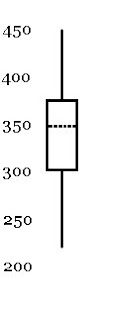
Here is a representation of five number summary above as a box and whisker plot. It could either be on a vertical scale, as pictured here, or it could be represented on a horizontal scale. When financial data from a set of time periods is summarized, the data is often represented with box and whiskers plots, though some websites call them candlesticks instead. The vertical scale represents the value in currency (usually dollars), while the horizontal scale represents the change in time, where the time periods can be any standardized amount, whether day to day or week to week or month to month.